Quantum driven Cognitive Computing
RQSA Theory – Develops algorithm for The QEXL Approach; overcoming limitations in gold standard Bayesian Network; while allowing for creation of generative models. Bayesian as such is an adaptive technique.
(March 8 2013, Version March 10 2013)
1. INTRODUCTION
1.1. Purpose and Background. The following document describes principle features of a mathematical system of practical importance in probabilistic ontology and semantics, and their applications inference and automated reasoning. Whilst applications are wide, healthcare may be the most pressing need [1]. The focus here is on aspects of practical importance in (a) decision support systems as Expert Systems (ES) derived from probabilistic rules formulated by experts, (b) decision support systems based on automated unsupervised data mining of structured data (DM), and (c) the Semantic Web (SW) and mining of unstructured data, here, essentially text analytics (TA). The primary areas of interest to the author is in Evidence Based Medicine (EBM), Comparative Effectiveness Research (CER), epidemiology, and Clinical Decision support Systems (CDSS), and bioinformatics, which provide useful reference points and test beds for more general application.
1.2. The Need for a New Approach. In general we are beset by a plethora of approaches for reasoning probabilistically when many probabilistic rules are available, and the same uncertainty about best practice poses problems for the SW to go probabilistic [2]. The easiest relations between things to handle probabilistically, i.e. to extract, quantify, and reason with, are “are associated with”, as in “A is associated with B and C and D” [2-6], and it has found many biomedical applications [7-14]. From many such and self probabilities or information, we can express “A if B and C and D” are readily derived. These are of course not the only relationships between things that we use when communicating information by natural language, but the latter are noteworthy in forming the basis of the Bayesian network or Bayes Net (BN) [15], which is a gold standard for probabilistic inference. It is theoretically well founded. However, the reason that we see a plethora of further approaches is that BN’s adherence to a strict set of axioms to avoid apparent difficulties makes it very restricted in application. A BN (one that is truly a BN by original definition confines) confines itself to use of conditional probabilities that reflect the above “if” relationship, to multiplicative operations implying just logical AND, it considers only one direction of conditionality when in general we are interested in inference about etiology or causes as well as outcomes, and not least it confines itself to acyclic directed graphs when networks of knowledge representation are in practice rich in cyclic paths. That last is because the ideal full treatment is a fully connected graph, not neglecting any relationship, which is necessarily dominated by cycles. Note that neglect of relationships by a BN is equivalent to saying that they are they are there with probability 1, and whilst to be fair to BNs it is true that this implies absence of information I = −log(P), it remains an extreme assumption that is evidently not justified when we consider the other conditional probability terms and in the context of all available data, often called the problem of coherence.
1.3. Advantages of the Present Approach. The advantages of the present approach can be referenced with respect to BN as the gold standard that does not traditionally provide the following.
(1) Bidirectional inference, i.e. etiologies as well as outcomes.
(2) Intrinsic treatment of coherence as Bayes Rule.
(3) Cyclic paths are allowed, fall out naturally as part of the theory, and do not require iteration.
(4) Not confined to AND logic
(5) Not confined to conditional probabilities. Relators and operators may be used symbolically albeit with probabilities, or as matrices or algorithms.
(6) Probability distributions represented by vectors.
(7) Metarules with binding variables such to generate new rules and evolve the old, evolving the old. Metarules are also used to define words from simpler vocabularies.
(8) Handling of negation and, when there are double negation etc., conversion to canonical forms.
(9) Reconciliation into one rule of rules that overlap in information content or are semantically equivalent, including reconciliation of their probabilities.
1.4. The Pursuit of Best Practice for the Theoretical Basis. Quantum mechanics (QM) claims to be a system of best practice for representing observations and for inference from them on all scales, although the notorious predictions by QM in the narrow band of scale of everyday human experience has discouraged investigation of applicability. This is due to the perception of QM as wave mechanics, even though we are not for everyday purposes usually interested in inference about waves. For that reason, the method is based more specifically on the larger QM of Paul A. M. Dirac [16-17] who established the theoretical basis of particle physics. Penrose [18] provides an excellent primer. That there is sufficient breadth to Dirac’s perception of QM to encompass semantics is indicated by Dirac’s Nobel Prize Banquet Speech in 1933, “The methods of theoretical physics should be applicable to all those branches of thought in which the essential features are expressible with numbers”. Dirac was certainly modestly referring to his extensions to physics as further extensible to human language and thought, because in interviews he explicitly excluded poetry and (more controversially) economics as subjective.
The author has published extensively in areas of some relevance, but the bibliography [19-31] refers to publications since 2005 which have some relevance to an idea first broached in Ref. [31]. The present report collates the observations that have survived as useful, adjusts some nomenclature as well as perceptions, and adds integrating material. “Best Practice” would be presumptive for these or indeed anyone’s publications (though “pursuit of Best Practice” validly reflects the intent). Indeed, these publications show various degrees of development from some naïve initial observations, and represent a learning curve, and so are presented in reverse chronological order. This is because whilst the author has some formal training as doctorates in, essentially, biophysics and theoretical and computational chemistry, the quantum mechanics of molecules then touched (and still does) only upon aspects related to pre-Dirac quantum mechanics. That pre-Dirac era is essentially that of Schrödinger that describes quantum mechanics as wave mechanics. It is based on the imaginary number i, the number such that ii = −1. The problematic wave nature arises because exponentials of i-complex values are periodic or wave functions: eiq = cos(q) + i sin(q). However, Dirac rediscovered another imaginary number, although it was first noted by Cockle in 1848 and relates to a broader Clifford calculus originating roughly around that time. It has very different consequences, as follows.
2. BASIC HYPERBOLIC COMPLEX INFERENCE
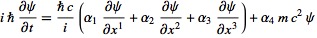
2.1. The Hyperbolic Imaginary Number. The “new” imaginary number is here represented as h such that hh = +1. Dirac developed what is now known as the Clifford-Dirac algebra. It, and h, arose in consideration of the origins of mass, introduced general relativity into quantum mechanical systems, and founded the current “standard model” of particle physics. Actually, the Clifford Dirac algebra and particle physics has several distinct imaginary numbers (that can all be represented as matrices). However they fall into the two general classes, of character i in that their squares are −1, and of character h in that their squares are +1. Otherwise, two different flavors of imaginary number are anticommutative, meaning that if the order is changed in which they form a product, the sign of the product changes. This includes hi = −ih. In the core theory presented here, different flavors of imaginary number do not meet up in the equations, and the focus is primarily upon h in isolation, meaning that focus is on purely hyperbolic complex or h-complex algebra (although real numbers are of course present, and that algebra sometimes delivers purely real-valued results, because hh = +1, and h−h = 0). In physics, those of h character include Dirac’s linear operator s, g0 (or gtime), and g5. Significantly for what follows, they particularly appear in physics as the equivalent to ½ (1+h) and ½ (1−h) multiplied by real or usually i-complex expressions, which are called spinors. As dual spinors in which these two spinors are involved, they relate to key expressions in quantum field theory, as well as the in theory discussed here.
2.2. The h-complex Hyperbolic Function. Unlike in i-complex algebra where eiq = cos(q) + isin(q), we are not usually concerned with making inference about waves, which may be important in physics and chemistry but not much in everyday life. As it happens, h is frequently called the hyperbolic number, and that is so because ehq is a hyperbolic, not a trigonometric and so periodic function (see next the Section after next for an interesting example and its physical consequences). We can express the h-complex hyperbolic function in the author’s notation (which will be valuable later below).
ehq = i*e−q + ie+q = cosh(q) + h sinh(q) (1)
where the notation means
i = ½ (1+h)
i* = ½ (1−h) (2)
For completeness and to demonstrate consistency with quantum mechanics, as well as for a few practical applications for present purposes (use of waves and wavelets), note that a somewhat more general description of quantum mechanics is given by
e+hiq = e−hiq = i*e−iq + ie+iq = cos(q) + hi sin(q) (3)
The full treatment following Dirac would be to resolve i into three kinds, one for each dimension of space, implying a Clifford-Dirac product of four imaginary numbers that leads to i = ½ (1+g5) and i* = ½ (1-g5), to same effect as g5 is a flavor of h: i.e. g5 g5 = +1. Although algebraically it does not of course matter, the author writes the i* term as the “lead term” i.e. as the focus of attention, for several reasons, one of which will become apparent later.
2.3. Complex Conjugation. The asterisk * used above and in other contexts below means forming the complex conjugate, i.e. changing the sign of the imaginary part, equivalent to replacing all +h by –h and vice versa. It is applied much more generally in the theory than just to rationalize i* and i*. Usually defined for i, we need to assume that it is extensible to h. However, in cases less relevant here where we need to think in terms of both imaginary numbers, note that we need to think of applying complex conjugation as (hi)* = ih = –hi, not h*i* = hi.
2.4. Physical and Statistical Interpretations. As indicated above, the relation to classical as opposed to wave behavior arises because ehq can be expressed in terms of hyperbolic functions. That means it can be expressed in terms of Gaussian functions (“normal distributions”) and their reciprocals by choice of variables in q. An example from physics is the choice of distance x = xt – x0 from starting point x0 in quantum mechanical expressions where a particle moves with momentum p=mx/t, giving q = -2pmx2/ht, with mass m, time t and Planck’s constant. Incidentally, Planck’s constant h is not of course be confused with the hyperbolic number h, and so when appearing elsewhere in discussions of physics the latter is usually written by the author in italic bold, as h, to make clear that distinction. The normalization procedure (Dirac recipe) is described later below, but for present purposes it suffices that the exponential of -2pmx2/ht is proportional to the probability of the absolute value |x|, and more generally, and as a practical application for the present context, it represents a normal distribution q = -½x2/s2 where starting point x0 becomes a mean value and √(ht/4pm) becomes the standard deviation s. The use of h does to some extent dictate a model of physical observation. To show consistency with quantum mechanics and interestingly consistency with the collapse of the wave function (e.g. Penrose reduction) interpretation, the above essentially suggests a kind of diffusion model, in which in isolation an i-complex description as a wave is the lowest energy state, but an observation of the particle as a particle and not a wave, or analogous physical perturbations, swings the description to a now lower energy h-complex one by “forcing the particle description”. This establishes a new x0 around which the particle collapses, although there is a accuracy of measurement conveyed by a standard deviation s in general, and at very least, for the most accurate measurements that are in principle possible, we have s = √(ht/4pm). Following the perturbation, the i-complex description is restored as the lowest energy state[1]. This relates to the physicists’ spread of the wave function, but it would be billions of years to see the phenomena for an object on the scale of a household object (by which time other entropic considerations would have had their effect). It is interesting to note that the collapse of the wave function seen this way does not necessarily imply a discontinuous i → h jump (or hi → i jump in the broader description of Eqn. 3) but a progressive rotation in time t or to an extent governed by the energy of the perturbation that may be interpretable as a field, of which demanding to measure it as a particle rather than wave is just a particularly strong case. The practical application here is that one can consider wave packets or wavelets that are progressively localized wave descriptions, and a Gaussian in the limit of being maximally localized. The applications outside of physics appear, however, to be in specialist areas such as probabilistic treatment of image analysis, and distributions generally are better described in terms of h-complex vectors, described later.
In consequence, we are considering the primary applications below as relating to the case when the parameters in q, and notably time, are fixed so that the exponentials merely relate to the single probability value such as P(A) of a state, event, observation, measurement or description A. P(A) that can empirically replace the concept of the exponential (as the statistical weight) and any normalizing factor for it. That said, the exponential form will make appearance in which the physicists’ q identifies with Fano’s mutual information I(A; B) between A and B, as described below, though we will also think of eI(A;B) as association constant K(A; B). The logarithm of the wave function y proportional to eq is seen as information that is somehow encoded. Note that eiI for any information I is a periodic function that bounds the different information and resultant probability values that one may have to the interval 0..2p. In contrast, ehI does not. h may be interpreted as adding the capacity for additional information that localizes the wave function as a Gaussian due to observations made, with a precision due to variance(i.e. square of standard deviation s2) as a counterpart of the physicists’ ht/4pm, which relates to the physicists’ notion of q as the action written in units of Plank’s constant h. For consistency with the physicist’s interpretation as wave function collapse due to loss and movement of information from the system, the treatment below should therefore be seen, reasonably enough, as the gain of information to the observer. In practice the information comes from sampling and counting of an everyday system as a population, or from our belief in the result that we would obtain by doing so.
2.5. Eigenvalues of h. Unlike the case of i that has imaginary eigenvalues +i and –i, we can also (as Dirac noted) replace h by its eigenvalues that are real, either +1, or −1. This is equivalent to treating i and i* as linear operators with eigenvalues 0 and 1, but specifically meaning that we can set i = 1 and i* = 0 to get one solution, and i = 0 and i* = 1 to get the other, giving two plausible physically real eigensolutions, or two sets of i-complex ones when expressions are also i-complex. Basic quantum mechanical texts gloss over this, jumping straight to e−iq and e+iq as the intuitive solutions and solving each separately, but Dirac made it clear by stating that a wave function is always decomposable into two parts, one a product with i and one a product with i* (although he didn’t use that notation). In physics, they typically relate to solutions in matters of direction in time or chirality (handedness) and more generally to direction in conditionality. That is meant in the same sense that conditional probability P(A|B) = PA, B)/P(B) is of reverse conditionality to P(B|A) = P(A, B)/P(A). In other words, the two eigensolutions do not imply indeterminacy in the sense that multiple eigenvalues would be possible interpretations. Rather, they simply relate to two directions of inference in the network and two directions corresponding of effect of the terms in it. However, we cannot compute P(A|B) from P(B|A) or vice versa by taking the adjoint † as the transpose and/or complex conjugate of either one of them because a classical probability is a scalar value, and has no imaginary part. In other words, P(A|B) is purely a symbolic adjoint of P(B|A). However, the effect of our i and i* operators is to render real values h-complex, and it should be held in mind that since (i)* = i* and (i*)* = i*, then (i*P(A|B) + iP(B|A))* = (i*P(B|A) + iP(A|B))*. Then given the (0,1) eigenvalues of these operators, we have P(A|B) and P(B|A) as the two eigensolutions.
2.6. Iota Algebra. Alternatively to thinking in terms of of Eqn. 3, one can for present purposes think of pre-Dirac quantum mechanics in which h replaces i, which in physics is called the Lorentz rotation, and it is arguably a generalization of the Wick rotation in which time t is replaced by imaginary time it to render quantum mechanical expressions classical. The resulting purely h-complex algebra takes some practice and excessive familiarity with i-complex algebra can sometime be more a hindrance than a help, because one can jump to conclusions that do not hold when h replaces i, and conversely miss important algebraic opportunities that h provides. Fortunately, h-complex algebra can be rendered in a form making manipulation much easier than in i-complex algebra. The above spinor forms, more generally quantities of form i*x and iywhere x and y are not h-complex, are so-called by analogy with Dirac’s treatment, and can be considered as comprising spinor operators i*and i with a very convenient algebra of their own. We can usually avoid discussion any of h by using them, i.e. by using i algebra or iota algebra alone. Its simple properties include the idempotent property ii = i and i*i* = i* which for example means that ei = i and ei* = i*, and similarly all powers and logarithms leave i or i* changed, but not of course the non-h-complex terms they multiply. They also include the annihilation property ii* = i*i = 0 that by annihilating terms in greatly facilitates multiplying h-complex expressions, and the normalization property i+i* = i*+i = 1, with the important effect that if a dual spinor form ix +i*y where x and y are real values, then ix +i*y = x + y. Note also that (ix +i*y)* = (i*y +i*x), important as the general statement that was implied in stating (i*P(A|B) + iP(B|A))* = (i*P(B|A) + iP(A|B))*. Eqns. 1 and 3 cover trigonometry and hyperbolic functions. That covers almost all the new algebra that we need here, but for completeness, because the Riemann zeta function z(s=1, n) = 1 + 2-s + 3-s +…+ n-s, is used in data mining and treatment of finite data to estimate information and probability values, it should be noted that z(x+hy, n) = i* z(x−y, n) + i z(x+y, n).
2.7. Dirac Notation. Let q be a function of A and B where are A and B are observed states or events that can take on particular values, being prepared that way, or by observation. More precisely, using the author’s notation, we should write A:=a and B:=b for these states or events as measurements. Here A and B are metadata or data descriptors such as momentum in physics or systolic blood pressure in medical life, and the specific values they have are a and b respectively, constituting the orthodata or specific manifestation of A and B. However, we can take A and B etc. as implying A:=a, B:=b etc. for brevity. We have, for example, in Dirac’s bracket or braket notation, where we can speak of a bra part <A| and a ket part |B>,
<A|B> = ke+hiq = ke−hiq = i*ke−iq + ike+iq = k(cos(q) + hi sin(q)) (4)
However, we shall assume that <A|B> is purely hyperbolic, i.e. there is a Lorentz rotation which here implies i → 1, and although this is not usually the case in quantum mechanical texts, a purely hyperbolic <A|B> is a valid solution. Above, k is a real valued constant dependent on the nature and scale of the system, and importantly it must be such that k relates to P(A) and P(B) meaning P(A:=a) and P(B:=b) so that the probability of a measurement value is purely one of chance without a prior observation of one of A and B, or in quantum mechanical language, without preparing a value of A or B. For example, in quantum mechanics texts considering a particle on a circular orbit of length L, we see k=1/L2.
2.8. Dirac Recipe for Observable Probabilities. The fact that we set a set a prior value of A and B, and then measure B or A as conditional upon it, means that that we think in terms of calculating P(A|B) and P(B|A), in quantum mechanics a process that algebraically implies first a ket |B> or bra |A> normalization as the preparation of B and A. We can write the bra normalized <A|B> as `<A|B> and the ket normalized<A|B>’, whatever that might mean algebraically at this stage. In fact, in the earlier example q = 2pmx2/ht, we are conceptually obliged to apply ket normalization since q = -2pmx2t/ht becomes q = +2pmx2/ht in the term ike+iq which can exceed an upper valid probability of 1 if t and m are, as in our everyday world, positive. Following Dirac’s recipe for observable probabilities we apply after ket normalization P(A|B) = <A|B>’ (<A|B>’)*, sometimes written as the square of the absolute magnitude |<A|B>|2 according to the Born rule but implying that <A|B> is ket normalized according to the Dirac recipe. In fact, the interpretation as |<A|B>|2 is peculiar to i-complex algebra and is not presumed here, and the more fundamental interpretation is that observation implies a projection operator P = |A><B| acting on vectors <A| or |B> (a vector interpretation is preserved in the current theory – see later below) such that
<A| P |B> = <A| |B><A| | B> = <A|B><B|A> = <A|B><A|B>* (5)
We cannot yet express <A|B> as a function of P(A|B) and P(B|A), but the solution must satisfy
<A|B> = i *<A|B> + i<A|B> = i *<A|B>’ + i ‘<A|B> = i *<A|B>’ + i (<A|B>’)*
= ‘<A|B> <A|B>’ (6)
P(A|B) =<A|B>’ (<A|B>’)* (7)
P(B|A) = ‘<A|B> (‘<A|B>)* = (<A|B>*)’ ((<A|B>*)’)* (8)
We can see the requirements for <A|B> emerging from the above by inspection, but when we apply it to Eqns. 1,3, and 4, we find that P(A|B) = P(B|A), which is the special case P(A) = P(B).
2.9. Conjugate and Non-Conjugate Variables. To move towards the required theory, we note that Eqns. 1,3, and 4 have a conjugate symmetry not suitable for our general and more classical purposes. That is, they are composed as i*x + iy. such that xy = 1 for all values of x and y. It arises because A:=a is a simple function f of B:=b and vice versa, so that the probabilities are predetermined as P(A:=a) = P(f(B:=b)) = P(f(A:=a)) = P(B). That is not generally true in quantum mechanics either, but relates to the important special case of conjugate variables such as momentum and position, or energy and time, and generally where the action A = (A:=a)(B:=b) such that q = 2pA/h. Classically, we can also be measuring values which are also such conjugate variables, like pressure P and volume V in the gas law PV = RT where R is a constant and when the absolute temperature T is constant, or current I and resistance R in the electrical engineering equation V= IR for constant voltage V. However, such cases in inference are rare, and in practice the extent to which P(A:=a) ≈ P(f(B:=b)) is more interesting as deducible from inference than as input, and moreover as part of a more general description of a relationship between A and B, i.eas the association constant
K(A; B) = P(A, B) / P(A)P(B) = eI(A; B) (9)
where I(A; B) is Fano’s mutual information, between A and B, noting K(A; B) = K(B; A) and I(A; B) = I(B; A).. We will generally only require for our applications that measurements and observations are such that 0 ≤ xy ≤ 1, and more specifically that 0 ≤ x ≤ 1 and 0 ≤ y ≤ 1, because we will relate them directly to empirical probabilities from data mining or human assignment. We can think of conjugate symmetry xy < 1 as the mother or prototype form, and we might say in physics that the dual spinor is a system in an asymmetric field that breaks the conjugate symmetry. Whilst this is most generally is of no relevance here, there is arguably one exception: an observation or measurement that implies the above described normalization as part of the Dirac recipe is an interaction analogous to an asymmetric field, and it sets one of x or y to 1.
2.10. The Braket as a Simple Linear Function of Empirical Probabilities. To all the above consideration there is only one and simple interpretation:
<A|B> = i*P(A|B) + i P(B|A) = [i *P(A) + iP(B)] K(A; B) = [i *P(A) + iP(B)] eI(A; B)
½ h[P(A|B) + P(B|A) + ½ h [P(B|A) – P(A|B)] (10)
which can be shown to satisfy Eqns. 6-9. Several things may be noted here and in Sections immediately following. First, we can see form the last line, analogous to the quantum mechanical Hermitian commutator form, that it is not entirely true that it is the only solution; we can replace +h by –h and satisfy most of the above discussion, with one exception, that in the case of conjugate variables it was argued that we must normalize the ket, not the bra, and that can be shown to imply Eqn. 10 as written. Second, specifically in the h-complex algebra, following the Dirac recipe does not suggest that we consider the square roots of probabilities in such expressions. In particular, our bra and ket normalizations become
<A|B>’ = i*P(A|B) + i (11)
‘<B|A> = i* + i P(B|A) (12)
Multiplying these by their own complex conjugates delivers P(A|B) and P(B|A) respectively. Computationally, is equivalent to using the following where Re and Im are the real and imaginary parts.
P(A|B) = Re<A|B> – Im<A|B> (13)
P(B|A) = Re<A|B> + Im<A|B> (14)
2.11. Classical Probabilistic Behavior. Above it was noted that h-complex functions exhibits classical local distribution functions.. The further point about Eqn. 10 is that it also yields classical probabilistic behavior. Notably for the chain rule P(A|C) ≈ P(A|B)P(B|C) and so P(C|A) ≈ P(C|A) that assume A and C independence, which is often physically the case, we obtain
<A|C> ≈ <A|B><B|C> = i*P(A|B)P(B|C) + iP(C|B)P(B|A)
= [i*P(A) + iP(B)] K(A; B) K(B; C) (15)
and similarly for <A|B><B|C><C|D> and so on.
2.12. Observation Brakets. There is an important special case of Eqns. 11 and 12 when A and B are statically independent, i.e. K(A; B) = 1, and when we are at least 100% sure that we are performing a preparation or measurement, which is here represented by ? where P(?) = 1. It gives us two terms which are the counterparts of prior self-probabilities in an inference network.
<B|?> = i * P(B|?) + i = i* P(B) + i (16)
<?|A> = i* + i P(A|?) = i* + i P(B) (17)
Note that the following t can be readily shown with a little standard algebra and recalling i *+ i = 1 so that i*x + ix = x ,
<?|A><A|B><B|C><C|D<D|E><E|?> = P(A, B)P(B, C)P(C,D)P(D|E) / P(B)P(C)P(D) (18)
which is an estimate of <A|E> = P(A|E), a joint probability that estimates the joint probability P(A, B, C, D, E).
2.13. Dirac Nets and Coherence. A network built from brakets (or bra-operator-kets – see later below) may be dubbed a Dirac Net. It is common as in Bayes Nets to consider a joint probability, although we can always make it conditional on say X or (X,Y) by dividing by P(X) and P(X, Y), which makes most sense of course when X and Y are states and events in the network. We can make a joint probability first by providing a full provision of observational brakets as all terminal nodes of the network, with a caveat as shortly to be mentioned. An advantage of Dirac Nets is that they can be used to ensure that the network is coherent with itself and all available data , meaning that all P(A|B)P(B) = P(B|A)P(A) and so on, which is Bayes Theorem. Ironically, Bayes Nets as usually defined as acyclic directed graphs do not consider this, since they only see one direction, P(A|B)P(B). If there is not such balance overall, or if it is conditional, and in a non-trivial way (e.g. missing probabilities are not 1), a Dirac Net value will have an imaginary part, positive or negative. In conversion of a Bayes Net to a Dirac Net, we will encounter branch points such as for example P(A| B, C) P(B|D)P(C|E). They allow that B and C are not independent in P(A| B, C) in one direction, but that they are independent in P(B|D)P(C|E) in the other direction. This will typically show up as a complex and not purely real value for a network. Consideration show that we need to correct this (arguable) mistreatment by a Bayes Net by multiplying by
<? ; B, C> = i* + iK(B; C) = <? | B, C> / <? | B > <? | C> (19)
Note that the construction <A|B><B|C> <B|D> etc., where we have a branch with two As, or indeed <C|A> <A|D> as a branch in the other direction, is valid. We need to correct accordingly in the first case by i* + i K(A; A) and in the second case by i*K(A; A) + i, where K(A; A) = P(A, A) / P(A)P(A). That is, by 1/P(A) if they are absolutely indistinguishable so that P(A, A) = P(A). But that is not necessarily the case if A is Bernoulli countable state, when P(A, A) = P(A)P(A).in that case no such correction is required. The general case of degrees of distinguishability is considered immediately after the following Section.
2.14. Cyclic Paths. Oddly, traditional Bayes Nets deny the possibility of cyclic paths, yet in a Dirac Net using observational brakets creates cyclic paths in order to get the answer we require. A full and proper use of observational brakets giving a purely real value indicates a joint probability, not a conditional one, but it applies whatever additional states, say F replace ?. Indeed it applies in replacement by two different states, say F and G, providing P(F) = P(G). It is an important feature of cyclic paths in an inference network formed by these methods that they are purely real, and appear to pose no special problems when a system is described where probabilities are in steady state, or sampled on a timescale much shorter than that over which it evolves. Such considerations show that <A|B><A|B>* = <A|B><B|A>* that yields observable probabilities is a simple case of such as cyclic path.
2.15. Distinguishability of States and Events. Actually, the simplest cyclic path is <A|A>. In quantum mechanics , texts often state that <A|A> = 1, but that is not in general true, and is just one possibility for the distinguishability of A and B on a continuum for <A|B> as a real line defined by P(A|B) = P(B|A), i.e. P(A) = P(B). <A|B> = 1 is the case when A and B are absolutely indistinguishable, so that P(A) = P(B) = 1, because P(A, A) =A. If they are distinguishable by recurrence so that the As can be counted, as when counting males in a population, then recurrences are independent (Bernoulli sampling) and <A|A> = P(A), because P(A,A) = P(A)P(A) Note here that <A, A, A | A> = P(A)3 and so on have meaning as concurrence of As. If A and B are totally indistinguishable, they are mutually exclusive, giving the orthogonal case, because P(A,B) = 0. Of course, many interesting cases do not satisfy P(A|B) = P(B|A), and we need to move from a real line to a plane, which can be described by a complex value. The valid region for probabilities in such a plane is in our case the h-complex iota space. It is contained by the vectors connecting the values 0 → i → 1 → i* → 0. With that, we are now ready to proceed to the ontological interpretation implying the verb to be, and on to other verbs and relationships in general, which will require a h-complex vector and matrix interpretation analogous to that in quantum mechanics.
3. HYPERBOLIC COMPLEX PROBABILISTIC SEMANTICS
3.1 Introduction and Overview of Agenda. Conditionality discussed in Section 1 is an example case of a relationship, but has several interpretations. Quantum mechanics does not well differentiate <B|A> from , since conditionality is typically seen as inevitably due to information relayed through cause and effect. The author uses “ontology” as closer to its older meaning of use of categorical relationships, i.e. the use of, in English, the verb “to be” and certain other related verbs as the relational operator or relator. More precisely, the term ontology is used here for the different interpretations of the relationship between nouns or noun phrases A and B in P(A|B) and <A|B>, that would reflect the way we sample to get counts that lead to the conditional probabilities. They can be distinguished by convenient readable choice of relator word or phrase in the form <A| relator |B> such as ‘if’. Whereas it is tempting, and indeed desirable to use symbols for ontological relators in particular, in applications natural language is used for readability.
Important examples follow. Here we shall not be too fussy about plurality of nouns and corresponding verb persons at present, although it can have effect in assigning probabilities. Rather, the more general existential notions of “some” and of the universal notions of “all” are the focus here(see later below). The asterisk that implies complex conjugation can for the moment be considered as used symbolically, to indicate and active-passive inversion of the relator on which it acts.
if* = implies (general conditionality)
when* = then (coincidence in time)
are* = include (categorical, set theoretic)
causes* = is caused by (causality)
“Semantics” is larger: it also includes other verbs such as verbs of action, where we have no choice but to write <A| relator |B> because there is way to construe that meaning by <A|B>. Other verbs primarily differ in the probabilities they convey, so the verb “to be” is regarded as the mother form from which they are derived. Meaning, in contrast, comes (a) from the h-complex probabilistic knowledge network of h-complex terms that specifies meaning as the network context, and (b) from definitions that are not fundamentally different in action from specifications of syllogisms and other logical laws, that evolve the network to generate new probabilistic statements.
In both ontological and full semantic treatment, we can think of the nodes such as A as states having self, marginal, or prior probabilities P(A), but they can also be viewed as parameters that set P(A|B) and P(B|A), as can be seen in Eqn. 10. Often that is the same thing, but we may not know these probabilities associated with the states as nodes, and subjectively at least, it is easier to assign conditional probabilities P(A|B) and P(B|A), from which P(A) and P(B) follow, given KA; B) = eI(A; B), the value of which can be changed to describe the probabilistic properties of different and diverse relationships. More correctly node probabilities are to be seen as h-complex values vectors of state |A> where we will equally well need <A|, but we can easily get <A| from |A>* as discussed below. The minimal perspective is that A and B are vectors of one lement, and more precisely the observational brakets discussed above, < ?|A> = i* + iP(A) = <A|?>* = (i*P(A) + iP(A))*. However they can be full vectors. Relators are operators that act on <A| or |B> first, to same effect, establishing the probability of the specified relationship. The development below is an agenda essentially follows symbolic manipulation → semiquantitative manipulation → symbolic projection with quantification → sufficient vectors→ distribution vectors. We can work at any stage on this continuum between symbolic and a full vector-matrix treatment.
3.2 Hermitian Operators as Relationship Operators. In general, any statements <A| relator |B> represent relationships in the network called probabilistic rules, or simply rules, that the applications import as XML-like tags. We can see a knowledge network as consisting of nodes or vertices A, B, C, that represent nouns and noun phrases as analogous to the physicists’’ states, or measurements concerning the actual values of states, and vertices between them as the relationships. The two pieces of relationship information in each direction of each edge are
<A| relator |B> = (20)
and
<B| relator |A> = <A| relator* |B> (21)
These two equations each individually represent the active-passive inverse form of the statement with no change in meaning, as in and <‘type 2 diabetes’ | is caused by | obesity>, where “is cause by” ≡ causes*. The two equations are connected by the complex conjugate of the whole rule:
* = (22)
So we can thing of a directed edge as associated with as a single complex value, encoding both directions of the relationship. The above define ontological and semantic relationships as Hermitian operators, an important class of QM operators related to data from observations and measurements. Were they not Hermitian, then * = *, as in * = <‘type 2 diabetes’ | is caused by | obesity>, which is true as active-passive inversion, an example of semantic equivalence, but it now loses the ability to represent two different directions of distinct effect, and in terms of the meaning, the graph is no longer a directed graph.
In the following few Sections, we would appear to be making use of the above symmetry rules in a way that is, if not exactly simply symbolic, nonetheless nominally quantitative. That this is not necessarily the case is discussed much later below. We shall focus first largely on the general semantic implications of the categorical case that is, after all extensible to verbs of action: = The two reasons why this not a good idea ouside of formulating the case with non-categorical verbs is that (a) it multiplies the number of nodes represented in states by having a variety of properties associated with each same noun, and (b) we will typically want to inference by referring to the object noun as a state, here cat, rather than to a quality of the subject noun, here dogs as cat-chasers.
3.3. Existential and Universal Quantification. In the ontological interpretation that is specifically categorical, <A|B> is translated as follows.
<A|B> = = = = <A| are B>* (23)
One consequence is that we can think of <A|B> in a very simple way.
= i P(“A are B”) + i*P(“B are A”)
= ½ [(“A are B”) + P(“B are A”)] + ½ h[[(“A are B”) − P(“B are A”)] (24)
Note that we have switched i and i * for a more readable styles, as it is nice that the first term iP(“A are B”) images . It is important to note that the existential notions of “some” and the universal notions of “all” are not required in these expressions, although they could be. Rather, they would relate to specific choices the values of P(“A are B”) and P(“B are A”) dictate that. When they are used, they follow a QM rule that is here applied to quantifiers such as ‘the’, ‘a’, ‘one’, ‘two’ ‘many’: when such an entity is moved outside the bra, its complex conjugate is taken (however, when moved outside the ket, it is unchanged.
< quantifier A | relator |B> = < A | quantifier* relator |B> (25)
< A | relator | relator |B> = < A | relator quantifier* relator |B> (26)
So, for example, = . So armed, we can express the extent of existential quantification as
= = Re<A| are |B> = ½ [(“A are B”) + P(“B are A”)] (27)
= Im <A| are |B> = ½ h[(“A are B”) − P(“B are A”)],
Im <A| are |B> > 0 (28)
= Im <A| are |B> = ½ h[(“A are B”) − P(“B are A”)],
Im <A| are |B> < 0 (29)
The above “greater than” or “less than” is for ease of interpretation, but it really represents a continuum, not a discontinuity. To put it another way, Im <A| are |B> reflects the universal case on a scale −1 to +1 mapping from “all A are B” to “all B are A”, and if is approximately zero , we can simply say that “some A are B” and no more. It is clear logical why the existential case subtends the universal: if all A are B, or all B are A, it necessarily follows that some A are B (and some B are A).
3.4. Trivially and Non-trivially Hermitian Relationships. More generally, relators are non-trivially Hermitian, because is not the same as in meaning or in probability. Or rather, they have that capacity, because a trivially Hermitian operator obeys the rules in Section 2.1. In addition, however, the latter obeys = as in < Jack | marries | Jill>, and note that whilst we can write “gets married by” = married*, here married = married*. Note that English often carries different meanings in verbs as if they were overloaded operators. Saying “the priest marries Jack and Jill” and even “the priest marries Jill” are not taken by the human reader as the same kind of meaning of “marries”, but we would need rules from the context to say that in the second case, considering whether in that religion priests can get married. The priest performs the ceremony of marriage, or “causes to be married”. Text analytics would need to perform context dependent task to distinguish the meaning, and we might say that a second operator holds with marries(2)* = ‘got married by’(2), but marries ≠ married*, so part of the distinct definition is that the verb is in the second meaning is not trivially Hermitian. We could write < The priest | causes | marriage> being careful that there is not another marriage performed by the priest in the same relevancy set of rules, and we note that causes and of are non-trivially Hermitian. For ‘of’, however, a categorical interpretation requires caution. In principle, we could say that aces of spades are the the same thing as the spades of aces, since the set of spades includes an ace, and vice versa. However ‘of’ carries linguistically an non-trivial Hermitian sense, of “owned by” or that in that B is a larger set of things than A. These difficulties vanish, to some extent, in the present system. Rather, <A| relator |B> quantifies the trivial or non-trivial nature of the spefiic relation in the context of a statement. It carries asymmetry as potentially different probabilities. P(Jack marries Jill”) = P(“Jill marries Jack”) but so <A| relator |B> is then purely real, but P(“The priest marries Jill”) > P(“Jill marries the priest”) even if neither can, a prior, be said to be said to probability 0 or 1.
3.5. Para-ontological Relationships. Note that
<A| are equivalent to |B> = <A|B> =<B|A> = = 1, if P(A|B) = P(B|A) (30)
In some sense, there is even a mother form of <A|B>, which is when A and B are seen together at random. Following Section 2.15, if there is no such association, such that A and B are independent, then <A|B> = P(A) P(B), and mutual information I(A; B) = 0 (i.e. K(A; B) = 1). Eqn. 10 then becomes, say,
= <A|B> = <B|A> = i*P(A) + i P(B)
= ( i*P(A) + i) ( i* + i P(B)) = <A|?><?|B> (31)
This lies in the scope of QM, but just means that we have the special case P(A) =P(A|B) and P(B|A) = P(A). By the Dirac recipe
<A|B>’ (<A|B>’)* = ( i*P(A) + i) ( i*P(A) + i) * = <A|?><?|A>
= ( i*P(A) + iP(A)) = P(A) (32)
But we are not confined to conjugate variables, and can bra-normalize.
‘<A|B> (‘<A|B>)* = ( i* + iP(B)) ( i*+ iP(B)) * <B|?><?|B> = P(B) (33)
In general <A|?><?|A> is not a relation but stands for the self probability P(A) of a node A in the network. There in this way no information describing the relationship, so this can be computed de novo as required from the self-probabilities P(A) and P(B) of nodes A and B. We do not need a rule (however, recall that its omission in a purely multiplicative network of which we wish to express the join probability implies that it is there with probability 1, not P(A)P(B)).
3.6. Negation. It must always be the case that <A|?><?|A> > 0 although to be pedantic we might say “providing A exists”. But it does not follow that <A|?><?|B> > 0. Note, then, the case when A and B are so distinguishable that they are mutually exclusive.
= <A|B> = 0 => = 1 (34)
It is the case of orthogonal vectors <A| and |B> discussed later below. This is actually an important case, because it is quite plausible to build a network in which nodes A, B, C, have distinct and non-overlapping meanings, or that some nodes in a network do. Cats and dogs can be nodes, and in the ontological interpretation = , evidently the value is zero. But it does not mean that, for example, is zero.
At first glance the rule, that when we move a quantifier outside of the bra we take the complex conjugate, at least symbolically, need not be applied here. That is because at first glance it seems that the words ‘no’, ‘not’, ‘none’ and ‘non-‘ do not obviously change the meaning when so moved, as if trivially Hermitian, e.g. not = not*. The situation is more subtle.
< no A | are |B> = < A | none are |B> = <A| are not |B> = <A| are |not B> =
= = = 1 (35)
The last equality = , which is not completely obvious to initial contemplation, is the logical law of the contrapositive. It includes, for example, “mammals are cats” ≡ “non-cats are non-mammals”, which takes a momen’s thought. But even more subtly, it holds quantitatively only under certainty, otherwise, using our original example, and can have different associated probabilities. Conversely we can see that does not have the same value as in any event, because while the latter is absolutely true as read, the former is only very occasionally true, in the sense that non-birds can be reptiles or fish, or trees etc. For these reasons we apply the out-of-bra and out-of-ket rules, and distinguish between
= <A| are |not B> =
= = <A| are not* |B> (36)
It may well be argued that these are not the same thing anyway, even to causal inspection, but then consistent with that, we are saying that ‘not*’ is different to ‘not’. The real point is it conveniently places the two distinct forms of negation within the relator phrase, i.e. as a property of the relationship.
3.7. Subjective Quantification as Semiquantitative Quantification. In several Sections following, how statements in a network interact depends on assigning probabilities that are valid combinations in that context, even if not necessarily true as reasonable estimates. If data is structured, even containing relationships, we can establish detailed probability values at least for that set of data. But reasonable estimates are of course desirable in every case, including textual and anecdotal statements about relationships, and need not be confined to the idea of an authoritative statement having probability 1 merely because the author stated it. This is harder, but probabilities are nonetheless constrained or guided in many examples considered so far. We could frequently at least say that forward and reverse values are equal, or one specified one is a lot larger than the other, but the other is definitely not zero. For example P(“cats are mammals”) = 1, while the reverse probability P(“mammals are cats”) is problematic. Consistent with the forward direction, it is reasonable that such probabilities relate to the size of sets they describe. For example, given that what you are sampling is a mammal, what is the chance of it being a cat, or what proportion of individual mammalian animals are also cats? Without any further conditions, this would require knowledge of the number of mammals and number of cats (number of individuals, not species). It is the kind of calculation that some people, and especially demographers, like to do as an exercise in indirect estimation. For example, in a detailed analysis Legay estimated 400 million cats in the world (although others estimate more than 500 million). Estimates of the number of mammalian species is relevant to estimating the number of individual mammals, and is around 6000 From that one guesses that the number of mammals, if cats were representative, is 400 x 6000 x 1000000 = 2.4 x 10¹². Importantly also, if the 6000 mammalian species were equally populated, we could then say that P(cats | mammals) = P(“mammals are cats”) ≈ 1/6000 ≈ 0. 00017. That gives some idea of the magnitudes if figures encountered, but assuming equal sized populations a bad assumption. Typically such distributions follow Zipf’s law that predicts that out of a population M of N elements, the probability P(e(k) | M) of elements of rank k is
P(e(k) | M) = (z(s, k) ̶ z(s, k ̶ 1)) / z(s, N) (37)
where we have written it maximally in terms of Riemann’s zeta function [3] defined as z(s, n) = 1 + 2 ̶ s + 3 ̶ s + …+ n ̶ s ). The zeta function has more general significance as the amount of information obtained by counting things. Although it does not immediately solve the P(cats | mammals) estimation problem, we note that P(cats | mammals) also estimated in terms of zeta functions is in our example case
P(cats | mammals) = ez(s=1, n[cats, mammals]) ̶ z(s=1, n[mammals]) = ez(s=1, n[cats]) ̶ z(s=1, n[mammals]) (38)
Here n[A] in general means “number of A”, i.e. the counted number, or observed frequency, of A. Note n[cats, mammals] = n[cats], since all cats are mammals. Putting the above together (along with, strictly speaking, considerations of the next Section) we have for 6000 mammalian species, and with cats ranked k[cats] as the k[cats] most populous species,
P(cats | mammals) = P(“mammals are cats”)
= ez(s=1, n[cats, mammals]) ̶ z(s=1, n[mammals])
= ez(s=1, n[cats]) ̶ z(s=1, n[mammals])
= (z(s, k[cats]) ̶ z(s, k[cats] ̶ 1) / z(s, N=6000)
= k[cats] ̶ s / z(s, N=6000)
logeP(cats | mammals) = z(s=1, n[mammals]) ̶ z(s=1, n[cats])
= s logek + loge z(s, N=6000)
For the simplest case of s = 1 and large amounts of data,
P(cats | mammals) = P(“mammals are cats”)
= ez(s=1, n[cats]) ̶ z(s=1, n[mammals])
≈ n[cats]) / n[mammals]
= (z(s, k[cats]) ̶ z(s, k[cats] ̶ 1) / z(s, N=6000)
= 1 / ( k[cats] ( loge(6000) + 0.5772))
z(s=1, n[mammals]) ̶ z(s=1, n[cats])
= logek + loge (loge z(s, N=6000) + 0.5772))
≈ logek + 2
where 0.5772… = g, the Euler-Mascheroni constant relating logarithms and zeta functions That loge ( loge z(s=1, N=6000) + 0.5772)) ≈ 2 is a reasonable approximation for a broad number of estimates of any number of taxonomic groups considered of which the group of specific interest, here domestic cats, is one: for N=100, it is more precisely 1.5, for N=1000,000, it is more precisely 2.6. We can note now that 1 ≤ k ≤ N, since it is the kth of the N groups. Hence logek cannot itself exceed the value of approximately 2 and so, again approximately, it lies in the range 0…2. For the 10th in the ranked list it would be about 0.8, for the 100th about 1.5, for the 1000th about 1.9, and for the 3000th (the median of the ranked list), it would be about 2.1. As a ball park estimate of what we expect for z(s=1, n[mammals]) ̶ z(s=1, n[cats]), we have z(s=1, n[mammals]) ̶ z(s=1, n[cats]) ≈ 4. In consequence,
P(cats | mammals) = P(“mammals are cats”) = ez(s=1, n[cats]) ̶ z(s=1, n[mammals]) ≈ 0.018.
However, we assumed s=1, and s can be critical in the Zip’s distribution. For large s and large N, z(s, N) → 1
P(cats | mammals) = P(“mammals are cats”)
= ez(s=1, n[cats]) ̶ z(s=1, n[mammals])
= (z(s, k[cats]) ̶ z(s, k[cats] ̶ 1) / z(s, N=6000)
= k[cats] ̶ s + 1
Hence
z(s=1, n[mammals]) ̶ z(s=1, n[cats])
= logek + loge (loge z(s, N=6000) + 0.5772))
≈ 2s, s >> 1
and so
P(cats | mammals) = P(“mammals are cats”) ≈ e ̶ 2s, s >> 1, and as reasoned earlier, P(cats | mammals) = P(“mammals are cats”) → ~ 0.018 when s → 1. Note that if we simply set s=1 in e ̶ 2s, then e ̶ 2 ≈ 0.14. The above 0.018 is two orders of magnitude higher than the value of 0.00017 reasoned even earlier above if all species in the Mammalia are equally densely populated, but that kind of qualitative disagreement is what may be expected by the more realistic distribution of mammalian species that we see, and by Zipf’s law. It suggests that s must be significantly greater than 1. More precisely, we have ̶ loge0. 00017 = 8.68 ≈ 2s, and so s ≈ 4.
3.9. Objective Treatment in Terms of Zeta Functions. The bases of the follow considerations are found in Refs. [3-6] and references therein. It is useful for calculations to note that we can rewrite Eqn. 10 in zeta function terms, with N as total data. Retaining expected frequencies, this is as follows.
<A|B> = [ i*P(A) + iP(B)]eI(A; B)
= [ i* ez(s=1, n[A]) ̶ z(s=1, N) + i ez(s=1,n[B]) ̶ z(s=1, N)] ez(s=1,n[A, B]) ̶ e[A, B])
= [ i* ez(s=1, n[A]) + i ez(s=1,n[B])] ez(s=1,n[A, B])] ̶ z(s=1, e[A, B]) ̶ z(s=1, N) (39)
Here e[ ] is an expected frequency, calculated on the classical, e.g.chi-square test basis: e[A, B] = n[A]n[B]/N = n[A]P(B) = P(A)n[B]. In the cat and mammal example, the above becomes
= i* ez(s=1, n[mammals]) + i ez(s=1,n[cats])]ez(s=1, n[cats, mammals]]) ̶ z(s=1,e[ cats, mammals]) e ̶ z(s=1, n[animals])
= i* ez(s=1, n[mammals]) + iez(s=1,n[cats])]e ̶ z(s=1,n[mammals]) ez(s=1, n[animals]) e ̶ z(s=1, n[animals])
= i* ez(s=1, n[mammals]) + iez(s=1,n[cats])]e ̶ z(s=1,n[mammals])
= i* + i ez(s=1,n[mammals]) ̶ z(s=1, n[cats]) (40)
The above estimate of P(cats | mammals) reflects the choice of z(s=1, n[cats, mammals]) ̶ z(s=1, n[mammals]) as the expected information E( I(mammals | cats) | D[cats, mammals]) given data D. Incidentally, note that n[cats, mammals] means n[cats & mammals], and the converse probability P(mammals | cats) =1 reflects the fact that we know that all cats are mammals, so we could replace n[cats, mammals]) by n[cats].
For what follows, note that we can get rid of the sometimes problematic total amount of data N by avoiding expected frequencies e[ ].
<A|B> = [ i*P(A|B) + iP(B|A)]
= [ i* ez(s=1, n[A, B]) ̶ z(s=1, n[B]) + i ez(s=1,n[A,B]) ̶ z(s=1, n[A] )
= [ i* e– z(s=1, n[B]) + i e–z(s=1,n[A])] ez(s=1,n[A, B])] (41)
3.10. Subjective Quantification. The two preceding Sections essentially addressed subjective and objective data, in that order. We can represent either, or combine both, as follows
Importantly, we can include expected frequencies of another kind [1,5,6], namely b[ ] that are based on subjective prior belief about the values.
<A|B> = [ i*P(A|B) + iP(B|A)]
= [ i* e– z(s=1, n[B])+b[B]) + i e–z(s=1,n[A])+b[A])] ez(s=1,n[A, B]+b[A, B])
≈ [ i* Be(A|B)e– z(s=1, n[A])+ iBe(B|A) e–z(s=1,n[B])] ez(s=1,n[A, B])] (42)
Here Be( ) are the pior, probability-like, degrees of belief, in the values, Be(A|B) = e– z(s=1, b[A|B]-b[A] and Be(B|A) = e– z(s=1, b[A|B]-b[A]. If we have zero objective (frequentist) information from counting, of course <A|B> = i* Be(A|B) + iBe(B|A). The use of Be( ) rapidly becomes a good approximation as the b[ ] increase; if any of their their values approach then the full zeta function representation should be used.
3.11. Chain of Effect. Further development benefits from the above quantitative and semi-quantitative ideas and the constraints imposed on the nature of the probabilities when used collectively in inference. Notably, when consider AB |B> CD |D> have to either assume that some kind of linker such as <B|C> orBC |C> has a value of approximately 1, or provide a linker. A note should be made here on why we care. After all, the example addresses little more than (a) establishing a web of relationships that help define nouns and noun-phrases, (b) can occasionally (albeit rarely) be important inference in deducing that dogs chase some mice-chasers, and (c) for <mice|?> establishing a collective truth of the statements. But there can be an important meaning when there is an implicit or explicit chain of effect. Categorical and causal relationships are a clear case of such. However, catching, transporting, selling, and eating fish can have important meaning as a chain of effect for an epidemiologist when one of several possible lakes are contaminated and the outcome is an incidence of food poisoning, and when they wish to establish most probable origins as well as predict outcomes. Indeed, every action exerted or something in the vicinity leaves some sort of trace on where and what it acts upon (e.g. culprit DNA), this being a principle of forensic science. Some are, however, more interesting than others. A large knowledge network may contain interesting and uninteresting cases from a probabilistic inference perspective, but even the uninteresting cases can affect the probabilities finally deduced from a joint probability that addresses a topic of interest. Those rules that are directly relevant constitute the relevancy set.
3.12. Symbolic Projection. There is an intermediate possibility between the scalar treatment so far, and the vector-matrix approach to follow. It is useful when probabilities are to be assigned by a human expert. For a more general relationship such as a verb of action, it is convenient to think of a symbolic projection of value from the operator into the bra and ket. It is an intermediate step towards a less extensively symbolic treatment.
<A| relator |B> = i* P(A:=relator, B:=relator*) + iP(B:=relator, A:=relator*)
= i* <A:=relator | B:=relator*> + i<B:=relator | A:=relator*> (41)
By thinking of the relator as “causes”, which is a kind of prototype action verb, we have a reference point allowing us to say the following under the causal interpretation of conditional probabilities as a joint probability.
<A| causes |B> = i* P(A:=causes, B:=causes*) + iP(B:=causes, A:=causes*)
= <B|A> = i* P(B|A) + iP(A|B)
(42)
That is, P(A|B) = P(B:=causes, A:=causes*). Consistent with this, <?|A><A| relatorAB |B><B| relatorBC |C><C|?> requires linkers such as i*P(B:=relator*) and iP(A:=relator*) to fill in gaps to complete the chain rule such as P(A|C) ≈P(A|B)P(B|C). Including links and associating then with appropriate brakets in a network intended to calculate a joint probability, it can readily be shown to be equivalent to using the following for each braket. It gives us Eqn. 41. <?|A><A| relatorAB |B><B| relatorBC |C><C|?> does not, as a consequence, contain redundant terms, and although Eqn. 35 is not conditional in its probabilities, it remains asymmetric and typically has an h-complex value. So in asking a human about the probability that A causes B and the probability for the converse, the question in this case is as to with what probability doogs doing chasing occurs with cats being chased, and the probability that cats doing chasing occurs with dogs being chased.
There is an algebra that links the metadata operator ‘:=’ to conditionality, e.g. P(mammals:=cats) = P(mammals | cats). It suggests P(A|B) = P(A:=causes, B:=causes*) = P(A , B | causes, causes*), but that is not correct because it loses the information as to which of A and B are the cause. It exemplifies the limitations of an approach that is still essentially in terms of conditional probabilities and <A|B>, when it is QM’s <A| operator |ket> that is needed.
3.13. Sufficient Vectors. The following has the limitation that it is only really suitable for (a) ontological relations (i.e. that are some kind of interpretation of <A|B>, not necessarily categorical), and (b) trivially Hermitian relators in general. Actually, the overall non-trivial Hermitian effect can be represented, but it is dependent on choosing particular different values for the probabilities P(A), P(B) etc. implied by the nodes. That may conflict with values that we want the nodes to have when engaged in other interactions. That <A| and |B> are vectors of at least two elements is not strictly true in the Dirac notation. The significance of the notation <A| and |A> is that one is the transpose of the other, but we add the requirement that one is also the complex conjugate of the other, and so the general requirement is,
<A| = |A>* (24)
The above double * and T consideration follows from the use of complex algebra (i-complex and h-complex) to represent directions of effect, as in <A|B> = <B|A>* and = *. But if x is a scalar real number, it is unchanged by the transpose when seen as a vector or matrix of one element, and unchanged by complex conjugation because its imaginary part is zero, and the Dirac notation as implying the above transformations means that
<x| = x* = x, |x> = x, (25)
On the other hand, it also follows that if we address a complex scalar value say x+hy where y is also a scalar real value,
< x+hy | = (x+hy)* = x−hy, | x+hy> = x+hy, (26)
Consistent with that, but not requiring that the vectors are of one element, we can think of the observation brakets as vectors (not necessarily of one element), and a projection matrix over the whole space as an identity matrix|?><!–?| = I, then times eI(A; B) To see the relation with QM for operator, we can write
<a| relator=”” |b=””> = <a| <b=””>|?><!–?| eI(A; B) |B> = <a| <b=””>I eI(A; B) |B> (27)
It is sufficient to think of vectors of one element <a| ==”” <a|<b=””>?> = i *P(A) + i, and |B> = <?|B> = i * + iP(B), because the above equation holds true for I = 1. Recall however that we can write <a|b> = [i *P(A) + iP(B)] eI(A; B) = <a|?> eI(A; B) <?|B>, so we can write
<a| relator=”” |b=””> = <a| e<sup=””>I(A; B) |B> = <a|?> eI(A; B) <?|B> = <a|b> (28)
What this curious equation means is that <a|?> eI(A; B) <?|B> is the case <a|?><?|B> for I(A; B) =0, and A and B are independent. In this case, the relator here inserts mutual information on A and B as independent. There is just a single eigenvalue, though we could consider that an relator implies a distinct eigenvalue from the space of all possible relators. In that sense we can represent the probabilistic effect of any relator I eI(A; B) just by inserting into <a|b> an exponential of a new I(A; B). We can accept any I(A; B) because it has the property of being independent of P(A) and P(B) respectively, since it abstracts them as in I(A; B) = lnP(A, B) – ln(A) – lnP(B). I(A; B) varies much less than P(A) and P(B) when used as a metric that is measured from on population and applied to another, including the population of a single patient for which we wish to perform inference as to best action. However, the limitations mentioned, at the beginning of this Section, hold.
3.14. Operators Acting on Orthogonal Sufficient Vectors. The following works for orthogonal vectors, i.e. when <a|b> = 0. The extent to which that is not actually a restriction is discussed below. Recall that [a, b; c, d] [p, q]T = [ap+bq, cp+dq]T is the product of a matrix with a column vector, and [p, q] [a, b; c, d] = [pa+qc, pb+qd] is the product of a row vector with a matrix. Let us first consider the matrix
Q(A, B) = [0, i eI(A;B) ; i*eI(A;B),0] = [0, i; i*,0] eI(A;B) (29)
withectors <a| and=”” |b=””> are of consistent form satisfying <a| ==”” |a=””>*.
|B> = [i*P(B), i)]T
<b| = =”” [<b=””>iP(B), i*]
<a| ==”” [<b=””>iP(A), i*] (30)
Q(A,B) |B> = [0, i eI(A;B) ; i*eI(A;B),0] [i*P(B), i)]T = [ie I(A;B), i*P(B) e I(A;B)]T (31)
<a| Q(A,B) |B> = [iP(A), i*] [iP(e I(A;B), i*P(B)e I(A;B)] T = iP(A)e I(A;B) + i*P(B)e I(A;B)
=i*P(A|B) +iP(B|A) (32)
This is not a restriction if we ensure that all relationships are of character. In other words, even for the basic ontological cases we use [0, i; i*,0] eI(A;B) as a joining operator, and one that stands for (using our English type notation of earlier) ‘if’, ‘whe’n,’ is caused by’, and ‘include’. If we want to have another relation we use a new I(A; B) to represent its different probabilities. This attempt has a serious problem, however, in the complex conjugates of the matrices the idempotent multiplications ii= i and i*i* = i*are replaced by the annihilations are ii* = i*i = 0, and so the net result is <a| Q(A,B) |B> = 0. We would be confined to replacing, for example by <b| include=”” |a=””>, because = <a| are=”” |b=””> = 0. Constructions like by <b| include=”” |a=””> are semantically equivalent in the categorical interpretation, but irksome and restricting. However, it has its uses, notably as the effective matrix with time dependent modifiers. For example,
<a| now=”” destroys=”” |b=””> = 1
= 0
This is beyond scope of the present introduction. For present purposes, it is good that we can prevent annihilation by using the matrix [0, i*+i eI(A;B) ; i*eI(A;B)+i,0] that leaves an idempotent multiplication. Using vectors
|B> = [i*, i P(B)]T
<a| ==”” [<b=””>i, i* P(A)] (33)
we have
R(A,B) |B> = [0, i*+i eI(A;B) ; i*eI(A;B)+i,0] [i*, i P(B)]T =[iP(B)e I(A;B), i*e I(A;B)]T (34)
<a| R(A,B) |B> = [i, i* P(A)] [iP(B)e I(A;B), i*e I(A;B)] T = iP(B)e I(A;B) + i*P(A)e I(A;B)
=i*P(A|B) +iP(B|A) (36)
We can again change I(A; B) to represent the probabilities involved in a new relationship.
3.15. Distribution Vectors. In general, the appearance of an operator implies in QM that it is a matrix and that we see <a| and=”” |b=””> as vectors between which the operator sits, and it can act on either <a| or=”” |b=””> first to same effect. Following QM exactly, we have
<a| = =”” [<a|y<sub=””>0>, <a|y1>, <a|y2>, ….] (32)
|B> = [<y0|B>, <y1|B>, <y2|BA>, ….]T (33)
which obey the general rules described in the next section with T here indication transposition to a column vector, and for which vector multiplication satisfies the QM law of composition of probability amplitudes (and exemplifies a kind of inference network).
<a|b> = Si = 0,1,2,3,…n<a|yi><yi||B> (34)
The problem is that in QM, y is the universal wave function (universal quantum state) to which the probabilities of all other states A, B, C, etc can be referred with high precision. To do that it represents a information repository with a trans-astronomic, indeed by definition, cosmological, number of bits 0,1,0,0,1,1,1,…In practice, QM practitioners focus not on the universe but a specific subsystem of interest. In our case, we need to choose an ubiquitous if not universal state that is of interest. The obvious one for A as, say, obesity, or diabetes type 2, or systolic blood pressure 140 mmHg, or systolic blood pressure greater than 140 mmHg, is that y is age, and the indices of y 0, y1, y2 are its value (how many years old). Whatever the base chosen (here age), vectors represent probability distributions when expressed as above, and so represent distribution vectors.
Use of matrices to act on such distributions is rare in our current applications and beyond scope of tis introduction. Note, however, that we can construct projection operators generally as Pi = 0,1,2,3,…n|yi><yi||. We can sum over many P to obtain a new P if their component ket and bra are not orthogonal, and the result is the identity operator I if we sum over the the whole larger space, not just n-dimensional, meaning we consider more elements than just the n elements in the above vectors. We can multiply a projection operator by the analogue of the exponential of mutual information to obtain an operator (which is not a projection operator, since the effect of including this exponential is that result squared does not return itself, but itself times the square of this exponential).
References
- Robson, B., and Baek, O.K. (2009) “The Engines of Hippocrates: From the Dawn of Medicine to Medical and Pharmaceutical Informatics” B. Robson and Ok Beak (2009), John Wiley & Sons
- http://publications.wim.uni-mannheim.de/informatik/lski/Predoiu08Survey.pdf
- Robson , B. (2003) “clinical and Pharmacogenomic Data Mining. 1. the generalized theory of expected information and application to the development of tools” J. Proteome Res. (Am. Chem. Soc.) 283-301, 2
- Robson, B., and Mushlin, R. (2004) “clinical and Pharmacogenomic Data Mining.. 2. A Simple Method for the Combination of Information from Associations and Multivariances to Facilitate Analysis, Decision and Design in Clinical Research and Practice. J. Proteome Res. (Am. Chem. Soc.) 3(4); 697-711
- Robson, B (2005) . Clinical and Pharmacogenomic Data Mining: 3. Zeta Theory As a General Tactic for Clinical Bioinformatics. J. Proteome Res. (Am. Chem. Soc.) 4(2); 445-455
- Robson, B. (2008) Clinical and Pharmacogenomic Data Mining: 4. The FANO Program and Command Set as an Example of Tools for Biomedical Discovery and Evidence Based Medicine” J. Proteome Res., 7 (9), pp 3922–3947
- Mullins, I. M., Siadaty, M. S., Lyman, J., Scully, K., Garrett, C. T., Miller, W. G., Robson, B., Apte, C., Weiss, S., Rigoutsos, Platt, D., Cohen, S., Knaus, W. A. (2006) “Data mining and clinical data repositories: Insights from a 667,000 patient data set” Computers in Biology and Medicine, Dec;36(12):1351-77
- Robson, B., Li, J., Dettinger, R., Peters, A., and Boyer, S.K. (2011), Drug discovery using very large numbers of patents. General strategy with extensive use of match and edit operations. Journal of Computer-Aided Molecular Design 25(5): 427-441 (2011)
- Svinte, M., Robson, B., and Hehenberger, H.(2007) “Biomarkers in Drug Dvelopment and Patient Care” Burrill 2007 Person. Med. Report. Vol. 6, 3114 – 3126. 8
- Robson, B. and McBurney, R. (2013) “The Role of Information, Bioinformatics, and Genomics” pp 77-94 in Drug Discovery and Development. Technology in Transition, Churcill Livingstone, Elsevier
- Robson, B (2013) “Rethinking Global Interoperability in Healthcare. Reflections and Experiments of an e-Epidemiologist from Clinical Record to Smart Medical Semantic Web” Johns Hopkins Grand Rounds Lectures http://webcast.jhu.edu/Mediasite/Play/ 80245ac77f9d4fe0a2a2 bbf300caa8be1d
- Robson, B. (2013)“Towards New Tools for Pharmacoepidemiology”, Advances in Pharmacoepidemiology and Drug Safety, 1:6, http://dx.doi.org/10.4172/2167-1052.100012, in press.
- Robson, B. and McBurney, R. (2012) “The Role of Information, Bioinformatics and Genomics”, pp77-94 In Drug Discovery and Development: Technology In Transition, Second Edition, Ed. Hill, R.G., Rang, P. Eds. Elsevier Press.
- Robson, B., Li, J., Dettinger, R., Peters, A., and Boyer, S.K. (2011), “Drug Discovery Using Very Large Numbers Of Patents. General Strategy With Extensive Use Of Match And Edit Operations”, Journal of Computer-Aided Molecular Design 25(5): 427-441 (2011)
- http://en.wikipedia.org/wiki/Bayesian_network
- http://en.wikipedia.org/wiki/Paul_Dirac
- Dirac,. P. M. (1930) “The Principles of Quantum Mechanics”, Oxford University Press.
- Penrose, R. (2004) “The Road to Reality: A Complete Guide to the Laws of the Universe”, Vintage Press
- Robson, B. “Schrödinger’s Better Patients”, Lecture and Synopsis University of North Carolina, http://sils.unc.edu/events/2012/better-patients (4/16/2012)
- Robson, B. (2012) “Towards Automated Reasoning for Drug Discovery and Pharmaceutical Business Intelligence”, Pharmaceutical Technology and Drug Research, 2012 1: 3 ( 27 March 2012 )
- Robson, B., Balis, UGC , and Caruso, T.P. (2012), “Considerations for a Universal Exchange Language for Healthcare, IEEE Healthcom ’11 Conference Proceedings, June 13-15, 2011, Columbia, MO pp 173-176
- Robson, B (2009), “Towards Intelligent Internet-Roaming Agents for Mining and Inference from Medical Data”, Studies in Health Technology and Informatics,
Vol. 149 pp 157-177
- Robson,B. (2009), “Links Between Quantum Physics and Thought (for Medical A.I. Decision Support Systems) ”, Studies in Health Technology and Informatics, Vol. 149, pp 236-248
- Robson. B (2009) “Artificial Intelligence for Medical Decisions” 14th Future of Health Technology Congress, MIT , September 29-30 2010 and Robson. B (2009) “Using Deep Models of Medicine and Common Sense to Answer ad hoc Clinical Queries” 14th Future of Health Technology Congress, MIT , September 28-29, 2009.
- Robson B., and Baek OK (2009), “The Engines of Hippocrates: From the Dawn of Medicine to Medical and Pharmaceutical Infromatics.” BOOK, 600 pages, pub. Wiley.
- Robson B., and Vaithilingam A. (2009) “Drug Gold and Data Dragons. Myths and Realities of Data Mining in the Pharmaceutical Industry” in Pharmaceutical Data Mining: Approaches and Applications for Drug Discovery, Ed. Konstantin V. Balakin, Pub. Wiley
- Robson B. (2008) “Clinical and Pharmacogenomic Data Mining: 4. The FANO Program and Command Set as an Example of Tools for Biomedical Discovery and Evidence Based Medicine” J. Proteome Res. (Am. Chem. Soc.). ” J. Proteome Res., 7 (9), pp 3922–3947
- Robson B., and Vaithilingam, A. (2008) “Protein Folding Revisited” in Molecular Biology and Translational Science, Vol. 84 Ed. Kristi A.S. Gomez., Elsevier Inc.
- Robson B. and Vaithilingam, A. (2007) A. “New Tools for Epidemiology, Data Mining, and Evidence Based Medicine”. Poster, 10th World Congress in Obstetrics & Gynecology, Grand Cayman, 2007.
- Robson, B. (2007) “Data Mining and Inference Systems for Physician Decision Support in Personalized Medicine”. Lecture and Circulated Report at the 1st Annual Total Cancer Care Summit, Bahamas 2007
- Robson B. (2007) “The New Physician as Unwitting Quantum Mechanic: Is Adapting Dirac’s Inference System Best Practice for Personalized Medicine, Genomics and Proteomics?” J Proteome Res. (Am. Chem. Soc.), Vol. 6, No. 8: pp 3114 – 3126
[1] It should be declared that a Gaussian function can also be reached within an i-complex description provided that we see a particle as a harmonic oscillator in the ground state, for which the wave function solution is well known to be a Gaussian function. The particle is then seen as oscillating around the fixed point x0. In that sense, h-complex quantum mechanical descriptions relate to ground state harmonic oscillations in the i-complex description, but do not explain why a wave and not particle is a lower energy state in the absence of perturbation (unless energy is withdrawn from the system by perturbation). However, the rest mass as a kind of ground state of motion in the Dirac equation for mass predicts the mass as due to an oscillation. Here the rest mass is computed via igtime ∂y/∂t where gtime is a hyperbolic number, suggesting the more general hi description as starting point.


You must be logged in to post a comment.