Month: December 2015

Probabilistic Modeling, Predictive Analytics & Intelligent Design from Multiple Medical Knowledge Sources

Bioingine.com; Probabilistic Modeling and Predictive Analytics Platform for A.I driven Deep Learning to discover Pathways from Clinical Data to Suggested Ontology for Pharmacogenomics; achieving Personalization and Driving Precision Medicine.

Data Integration in the Life Sciences: 11th International Conference, DILS 2015, Los Angeles, CA, USA, July 9-10, 2015, Proceedings

The Feature Diagram from the book above:-

Pharmacogenomic knowledge representation, reasoning and genome-based clinical decision support based on OWL 2 DL ontologies

Combining Multiple knowledge Sources and also Ontologies:-

[Suggested Ontologies for Pharmacogenomics converging to help find a Pathway]

Patient Data (HL7, C-CDA)
Gene Ontology
ChEBI Ontology

Integration of Knowledge for Personalized Medicine:- Pharmacogenomics case-study

Looking Forward: The Case for Intelligent Design (and Infrastructure) in Life Science Biologics R&D Sponsored by: Dassault Systèmes; Alan S. Louie, Ph.D. January 2015

http://gate250.com/tc2/IDC%20Biologics%20White%20Paper.pdf

Clinical Decisions and Empirical Dilemma :- Priori Knowledge independent of Experience vs Posterior Knowledge dependent on Experience

Leon Festinger, American social psychologist, is credited to have developed the idea around Cognitive Dissonance

As such evidence in Evidence Based Medicine is sought and built around empirical evidence, as experienced and commonly observed, the dilemma is that this empirical evidence has the hazard of being fraught with cognitive dissonance.

Bioingine.com employs algorithmic approach based on Hyperbolic Dirac Net that allows inference nets that are a general graph (GC), including cyclic paths, thus surpassing the limitation in the Bayes Net that is traditionally a Directed Acyclic Graph (DAG) by definition.

The Bioingine.com approach thus more fundamentally reflects the nature of probabilistic knowledge in the real world, which has the potential for taking account of the interaction between all things without limitation, and ironically this more explicitly makes use of Bayes rule far more than does a Bayes Net. It also allows more elaborate relationships than mere conditional dependencies, as a probabilistic semantics analogous to natural human language but with a more detailed sense of probability.

To identify the things and their relationships that are important and provide the required probabilities, the Bioingine.com scouts the large complex data of both structured and also information of unstructured textual character. It treats initial raw extracted knowledge rather in the manner of potentially erroneous or ambiguous prior knowledge, and validated and curated knowledge as posterior knowledge, and enables the refinement of knowledge extracted from authoritative scientific texts into an intuitive canonical “deep structure” mental-algebraic form that the Bioingine.com can more readily manipulate.

Empiricity has the hazard of introducing Cognitive Dissonance.

Why “Science”-Based Instead of “Evidence”-Based?

The rationale for making medicine more science-based

https://www.painscience.com/articles/ebm-vs-sbm.php

A priori and a posteriori

From above link:-

The Latin phrases a priori ( “from the earlier”) and a posteriori ( “from the latter”) are philosophical terms of art popularized by Immanuel Kant‘s Critique of Pure Reason (first published in 1781, second edition in 1787), one of the most influential works in the history of philosophy.[1] However, in their Latin forms they appear in Latin translations of Euclid‘s Elements, of about 300 bc, a work widely considered during the early European modern period as the model for precise thinking.

These terms are used with respect to reasoning (epistemology) to distinguish necessary conclusions from first premises (i.e., what must come before sense observation) from conclusions based on sense observation (which must follow it). Thus, the two kinds of knowledge, justification, or argument[clarification needed] may be glossed:

A priori knowledge or justification is independent of experience, as with mathematics (3+2=5), tautologies (“All bachelors are unmarried”), and deduction from pure reason (e.g., ontological proofs).[3]
A posteriori knowledge or justification is dependent on experience or empirical evidence, as with most aspects of science and personal knowledge.

There are many points of view on these two types of knowledge, and their relationship is one of the oldest problems in modern philosophy.

The terms a priori and a posteriori are primarily used as adjectives to modify the noun “knowledge” (for example, “a priori knowledge”). However, “a priori” is sometimes used to modify other nouns, such as “truth”. Philosophers also may use “apriority” and “aprioricity” as nouns to refer (approximately) to the quality of being “a priori“.[4]

https://en.wikipedia.org/wiki/A_priori_and_a_posteriori

Although definitions and use of the terms have varied in the history of philosophy, they have consistently labeled two separate epistemological notions. See also the related distinctions: deductive/inductive, analytic/synthetic, necessary/contingent.

(more…)

Kahneman, the recipient Nobel prize (with Tversky and others) provided important insights concerning Clinicians decision-making under uncertainty

Probabilistic reasoning and clinical decision-making: do doctors overestimate diagnostic probabilities?

“Clinicians make decisions in the face of uncertainty. Kahneman, the recipient of this year’s Nobel prize, (with Tversky and others) provided important insights concerning judgment and decision-making under uncertainty.1,,2 In order to deal with uncertainty, doctors often over-emphasize the importance of diagnostic tests, at the expense of the history and physical examination, believing laboratory tests to be more accurate.3 This ignores the fact that medical tests are far from being perfect or innocuous. The inappropriate use of diagnostic tests also contributes to the growing cost of medical care.”

http://www.nobelprize.org/mediaplayer/?id=531

Semantic Data Lake Delivering Tacit Knowledge – Evidence based Clinical Decision Support

Can the complexity be removed and tacit knowledge delivered from the plethora of the medical information available in the world.

” Let Doctors be Doctors”

Semantic Data Lake becomes the Book of Knowledge ascertained by correlation and causation resulting into Weighted Evidence

Characteristics of Bioingine.com Cognitive Computing Platform

Architecture style moves from Event driven into Semantics driven
Paradigm shift in defining system behavior – it is no more predicated and deterministic – Non Predicated Design
Design is “systemic” contrasting the technique such as objected oriented based design, development and assembling components
As such a system is better probabilistically studied.
Design is context driven, where the boundary diminishes between context and concept
System capability is probabilistically programmed by machine learning based on A.I, NLP and algorithms driven by ensemble of Math
Design based on Semantic mining and engineering takes precedence to complex event processing (CEP). CEP and Event Driven Architecture (EDA) are the part of the predicated system design. Business rules engine may be an overkill.
Ontology is created driven by both information and numbers theory

–Algebra – relationship amongst variables

–Calculus – rate of change in variable and its impact on the other

–Vector Space – study of states of the variables

Bioingine.com algorithm design driven by Probabilistic Ontology

Probabilistic Ontology characterizes the ecosystem’s behavior
Complex System’s semantic representation evolves generatively
System better represented by semantic multiples. Overcomes the barrier of Triple Store (RDF)
Human’s interact with the system employing knowledge inference technique
Inductive knowledge precedes knowledge by deduction

Bioingine.com is a Probabilistic Computing Machine

System’s behavior better modeled by the employ of probability, statistics and vector calculus (Statistics based on HDN an advancement to Bayes Net, where acyclic in DAG is overcome)
Generally the system is characterized by high dimensionality in its data set (variability) in addition to volume and velocity.
Most computing is in-memory

BioIngine.com; is designed based on mathematics borrowed from several disciplines and notably from Paul A M Dirac’s quantum mechanics. The approach overcomes many of the inadequacies in the Bayes Net that is based on the directed acyclic graph (DAG). Like knowledge relationships in the real word, and as was required for quantum mechanics, our approaches are neither unidirectional nor do they avoid cycles.

Bioingine.com Features –

Bi-directional Bayesian Probability for knowledge Inference and Biostatistics (Hyperbolic complex).
Built upon medical ontology (in fact this is discovered by machine learning, AI techniques).
Can be both hypothesis and non-hypotheses driven.
Quantum probabilities transformed to classical integrating vector space, Bayesian knowledge inference, and Riemann zeta function to deal with sparse data and finally driven by overarching Hyperbolic Dirac Net.
Builds into web semantics employing NLP. (Integrates both System Dynamics and Systems Thinking).

Framework of Bioingine –Dirac-Ingine Algorithm Ensemble of Math

Q-UEL & HDN (More Info click the link)

Clinical Data Analytics – Loss of Innocence (Predictive Analytics) in a Large High Dimensional Semantic Data Lake

From Dr. Barry Robson’s notes:-

Is Data Analysis Particularly Difficult in Biomedicine?

Looking for a single strand of evidence in billions of possible semantic multiple combinations by Machine Learning

Of all disciplines, it almost seems that it is clinical genomics, proteomics, and their kin, which are particularly hard on the data-analytic part of science. Is modern molecular medicine really so unlucky? Certainly, the recent explosion of biological and medical data of high dimensionality (many parameters) has challenged available data analytic methods.

In principle, one might point out that a recurring theme in the investigation of bottlenecks to development of 21st century information technology relates to the same issues of complexity and very high dimensionality of the data to be transformed into knowledge, whether for scientific, business, governmental, or military decision support. After all, the mathematical difficulties are general, and absolutely any kind of record or statistical spreadsheet of many parameters (e.g., in medicine; age, height, weight, blood-pressure, polymorphism at locus Y649B, etc.) could, a priori, imply many patterns, associations, correlations, or eigensolutions to multivariate analysis, expert system statements, or rules, such as jHeight:)6ft, Weight:)210 lbs> or more obviously jGender:)male, jPregnant:)no>. The notation jobservation> is the physicists’ ket notation that forms part of a more elaborate “calculus” of observation. It is mainly used here for all such rule-like entities and they will generally be referred to as “rules”.

As discussed, there are systems, which are particularly complex so that there are many complicated rules not reducible to, and not deducible from, simpler rules (at least, not until the future time when we can run a lavish simulation based on physical first principles).

Medicine seems, on the whole, to be such a system. It is an applied area of biology, which is itself classically notorious as a nonreducible discipline.

In other words, nonreducibility may be intrinsically a more common problem for complex interacting systems of which human life is one of our more extreme examples. Certainly there is no guarantee that all aspects of complex diseases such as cardiovascular disease are reducible into independently acting components that we can simply “add up” or deduce from pairwise metrics of distance or similarity.

At the end of the day, however, it may be that such arguments are an illusion and that there is no special scientific case for a mathematical difficulty in biomedicine. Data from many other fields may be similarly intrinsically difficult to data mine. It may simply be that healthcare is peppered with everyday personal impact, life and death situations, public outcries, fevered electoral debates, trillion dollar expenditures, and epidemiological concerns that push society to ask deeper and more challenging questions within the biomedical domain than routinely happen in other domains.

Large Number of Possible Rules Extractable a Priori from All Types of High-Dimensional Data

For discovery of relationships between N parameters, there are almost always x (to the power N) potential basic rules, where x is some positive constant greater than unity and which is characteristic of the method of data representation and study. For a typical rectangular data input like a spreadsheet of N columns,

[2 to the power of N] – N – 1 = X numbers of tag rules from which evidence requires being established. Record with 100 variables and joint probability 2 means;

2^100-100-1 = 1.267650600228229401496703205275 × 10^30

Evidence based Medicine driven by Inferential Statistics – Hyperbolic Dirac Net

http://sociology.about.com/od/Statistics/a/Introduction-To-Statistics.htm

From above link

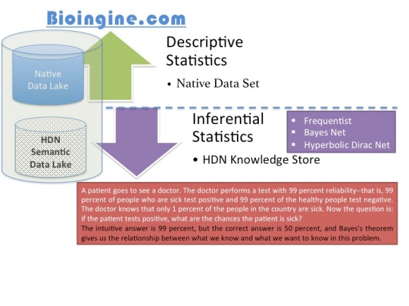
Descriptive Statistics (A quantitative summary)

Descriptive statistics includes statistical procedures that we use to describe the population we are studying. The data could be collected from either a sample or a population, but the results help us organize and describe data. Descriptive statistics can only be used to describe the group that is being studying. That is, the results cannot be generalized to any larger group.

Descriptive statistics are useful and serviceable if you do not need to extend your results to any larger group. However, much of social sciences tend to include studies that give us “universal” truths about segments of the population, such as all parents, all women, all victims, etc.

Frequency distributions, measures of central tendency (mean, median, and mode), and graphs like pie charts and bar charts that describe the data are all examples of descriptive statistics.

Inferential Statistics

Inferential statistics is concerned with making predictions or inferences about a population from observations and analyses of a sample. That is, we can take the results of an analysis using a sample and can generalize it to the larger population that the sample represents. In order to do this, however, it is imperative that the sample is representative of the group to which it is being generalized.

To address this issue of generalization, we have tests of significance. A Chi-square or T-test, for example, can tell us the probability that the results of our analysis on the sample are representative of the population that the sample represents. In other words, these tests of significance tell us the probability that the results of the analysis could have occurred by chance when there is no relationship at all between the variables we studied in the population we studied.

Examples of inferential statistics include linear regression analyses, logistic regression analyses, ANOVA, correlation analyses, structural equation modeling, and survival analysis, to name a few.

Inferential Statistics:- Bayes Net [Good for simple Hypothesis]

“Suppose that there are two events which could cause grass to be wet: either the sprinkler is on or it’s raining. Also, suppose that the rain has a direct effect on the use of the sprinkler (namely that when it rains, the sprinkler is usually not turned on)… The joint probability function is: P(G, S, R) = P(G|S, R)P(S|R) P(R)”. The example illustrates features common to homeostasis of biomedical importance, but is of interest here because, unusual in many real world applications of BNs, the above expansion is exact, not an estimate of P(G, S, R).

Inferential Statistics: Hyperbolic Dirac Net (HDN) – System contains innumerable Hypothesis

HDN Estimate (forward and backwards propagation)

P(A=’rain’) = 0.2 # <A=’rain’ | ?>

P(B=’sprinkler’) = 0.32 # <B=’sprinkler’ | ?>

P(C=’wet grass’) =0.53 # <? | C=’wet grass>

Pxx(not A) = 0.8

Pxx(not B) = 0.68

Pxx(not C) = 0.47

# <B=’sprinkler’ | A=’rain’>

P(A, B) = 0.002

Px(A) = 0.2

Px(B) = 0.32

Pxx(A, not B) = 0.198

Pxx(not A, B) = 0.32

Pxx(not A, not B) = 0.48

#<C=’wet grass’|A=’rain’,B=’sprinkler’>

P(A,B,C) = 0.00198

Px(A, B) = 0.002

Px(C=’wet grass’) =0.53

Pxx(A,B,not C) = 0.00002

End

Since the focus in this example is on generating a coherent joint probability, Pif and Pif* are not included in this case, and we obtain {0.00198, 0.00198} = 0.00198. We could us them to dualize the above to give conditional probabilities. Being an exact estimate, it allows us to demonstrate that the total stress after enforced marginal summation (departure from initial specified probabilities) is very small, summing to 0.0005755. More typically, though, a set of input probabilities can be massaged fairly drastically. Using the notation initial -> final, the following transitions occurred after a set of “bad initial assignments”.

P (not A) = P[2][0][0][0][0][0][0][0][0][0] = 0.100 -> 0.100000

P (C) = P[0][0][1][0][0][0][0][0][0][0] = 0.200 -> 0.199805

P ( F,C) = P[0][0][1][0][0][1][0][0][0][0] = 0.700 -> 0.133141

P (C,not B,A) = P[1][2][1][0][0][0][0][0][0][0] = 0.200 -> 0.008345

P (C,I,J,E,not A) = P[2][1][0][1][0][0][0][1][1][0] = 0.020 -> 0.003627

P (B,F,not C,D) = P[0][1][2][1][0][1][0][0][0][0] = 0.300 -> 0.004076